Performance
Historical Phoenix performance comparisons and feature-level improvements for scans, salting, and query execution.
This page has not been updated recently and may not reflect the current state of the project.
Phoenix follows the philosophy of bringing the computation to the data by using:
- coprocessors to perform operations on the server-side thus minimizing client/server data transfer
- custom filters to prune data as close to the source as possible.
In addition, to minimize startup costs, Phoenix uses native HBase APIs rather than going through the MapReduce framework.
Phoenix vs related products
Below are charts showing relative performance between Phoenix and some other related products.
Phoenix vs Hive (running over HDFS and HBase)
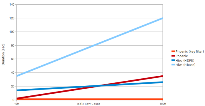
Query: SELECT COUNT(1) from a table over 10M and 100M rows. Data has 5 narrow columns. Number of region
servers: 4 (HBase heap: 10GB, processor: 6 cores @ 3.3GHz Xeon).
Phoenix vs Impala (running over HBase)
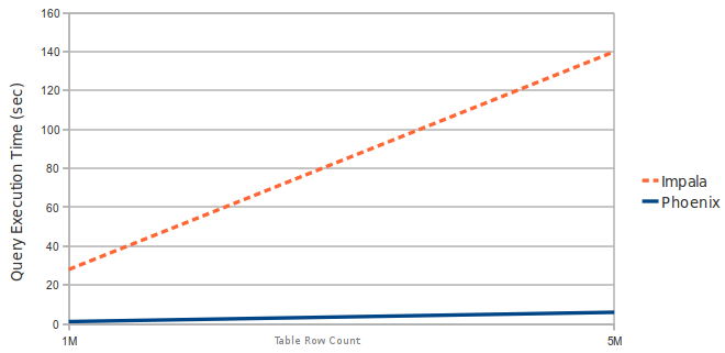
Query: SELECT COUNT(1) from a table over 1M and 5M rows. Data has 3 narrow columns. Number of region servers: 1 (virtual machine, HBase heap: 2GB, processor: 2 cores @ 3.3GHz Xeon).
Latest Automated Performance Run
Latest Automated Performance Run | Automated Performance Runs History
Performance improvements in Phoenix 1.2
Essential Column Family
The Phoenix 1.2 query filter leverages the HBase Filter Essential Column Family feature. This improves performance when Phoenix filters data split across multiple column families (CFs) by loading only essential CFs first. In a second pass, all CFs are loaded as needed.
Consider the following schema in which data is split into two CFs:
CREATE TABLE t (k VARCHAR NOT NULL PRIMARY KEY, a.c1 INTEGER, b.c2 VARCHAR, b.c3 VARCHAR, b.c4 VARCHAR).
Running a query similar to the following shows significant performance gains when a subset of rows matches the filter:
SELECT COUNT(c2) FROM t WHERE c1 = ?
The following chart shows in-memory query performance for the query above with 10M rows on 4 region servers, when 10% of rows match the filter. Note: cf-a is approximately 8 bytes and cf-b is approximately 400 bytes wide.
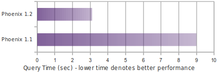
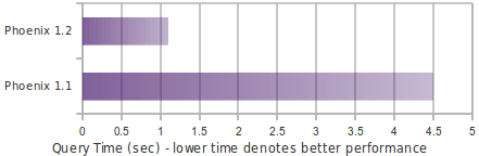
Skip Scan
Skip Scan Filter leverages HBase filter SEEK_NEXT_USING_HINT (docs). It significantly improves point queries over key columns.
Consider the following schema in which data is split into two CFs:
CREATE TABLE t (k VARCHAR NOT NULL PRIMARY KEY, a.c1 INTEGER, b.c2 VARCHAR, b.c3 VARCHAR).
Running a query similar to the following shows significant performance gains when a subset of rows matches the filter:
SELECT COUNT(c1) FROM t WHERE k IN (1% random k's)
The following chart shows in-memory query performance of the query above with 10M rows on 4 region servers when 1% random keys over the full key range are passed in the IN clause. Note: all VARCHAR columns are approximately 15 bytes.
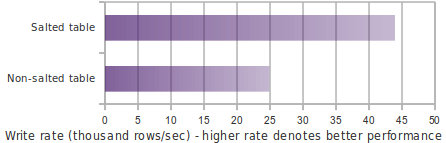
Salting
Salting in Phoenix 1.2 improves both read and write performance by adding an extra hash byte at the start of the key and pre-splitting data into regions. This reduces hotspotting on one or a few region servers. Read more about this feature here.
Consider the following schema:
CREATE TABLE T (HOST CHAR(2) NOT NULL,DOMAIN VARCHAR NOT NULL,
FEATURE VARCHAR NOT NULL,DATE DATE NOT NULL,USAGE.CORE BIGINT,USAGE.DB BIGINT,STATS.ACTIVE_VISITOR
INTEGER CONSTRAINT PK PRIMARY KEY (HOST, DOMAIN, FEATURE, DATE)) SALT_BUCKETS = 4.
The following chart shows write performance with and without salting, where the table is split into 4 regions on a 4-region-server cluster (note: for optimal performance, salt bucket count should match region server count).
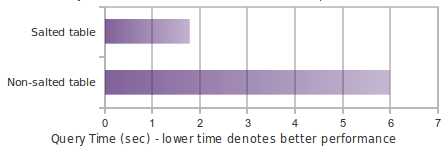
The following chart shows in-memory query performance for a 10M-row table where host='NA' matches 3.3M rows.
select count(1) from t where host='NA'
Top-N
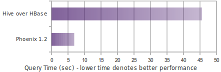
The following chart shows in-memory query time for a Top-N query over 10M rows using Phoenix 1.2 and Hive over HBase.
select core from t order by core desc limit 10